Genomics and bioinformatics data often are generated at many hierarchical levels. For example, an RDP 11classification of a 16S rRNA experiment yields calls to phylum, class, order, family and then genus with each level nested within the one above it. So a phylum can have many classes, which in turn can have many orders and so forth. For an rna-seq experiment on bacteria, reads can be mapped to genes, which in turn can be grouped into operons, with one to many genes per operon. In performing inference, it is not trivial to interpret these multiple levels. Typically, levels are chosen ahead of time and infernence is constrained to that level. For example, it is common to perform RDP analyses at the genus or phyla level. But such a priori filtering of the data may miss important patterns; for example, for some taxa a difference at the genus level might be important, while for other taxa in the same experiment, a meaningful signal won’t be observed unless a less derived phylogenetic level is considered.
In order to visualize such cases, this web page contains a demonstration project for visualization of
phylogenetic trees. In this example
we consider RDP classifications of a
previously published experiment.
This was a 454-based 16S rRNA experiment in which punch biopsies were collected from 33 subjects with
adenomas and 38 (control) subjects without adenomas.. In the analysis presented on this web page,
578,096 sequences were run through the stand-alone version of the RDP classifier (version 2.6).
Classifications to each phylogenetic level (phylum, class, order, family, genus) were taken if
the bootstrap value was >= 50. For each taxa at each level in the tree, a t-test was performed
testing the null hypothesis that the log-normalized distribution of that taxa was the same in
case vs. control.
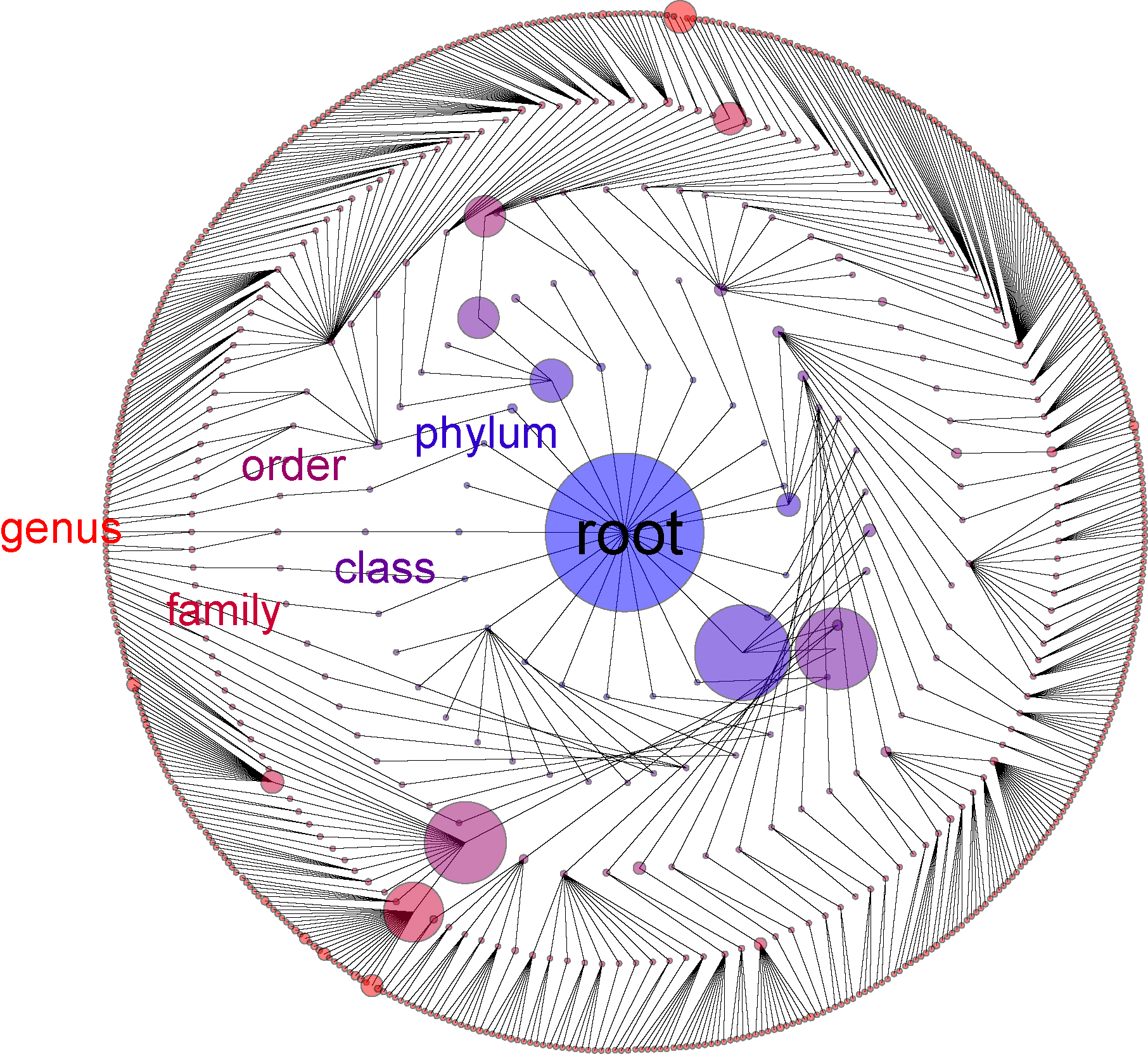
The visualization shown here (for Chrome
browsers only) shows the phylogenetic tree that results from this analysis. By default, the size of
each circle is the number of sequences assigned to each node:
If in the demonstration we hover the mouse over each of the large dots at the phylum level, we see that the three most abundant phyla in our samples were Phylum Firmicutes (with 340,933 sequences), Phylum Bacteroidetes (with 142,231 sequences) and Phylum Proteobacteria (with 67,926 sequences) as we might expect from a human gut micro-environment.
One of the nice things about the demonstration is that we can switch between a traditional circular phylogenetic tree (as in the figure above) and a Force Tree view. We can do this by clicking on the "reanimate" button in the left hand control panel. On hitting this button, we switch to a view in which opposing forces position each node. These forces include "gravity" which tends to pull each node to the center of the screen, a repulsive focce between each node and an elastic spring-like force that in this case reflects the phyologentic distance between different taxonomic levels (so for example the distance between genus and family will be shorter than the distance between genus and order):
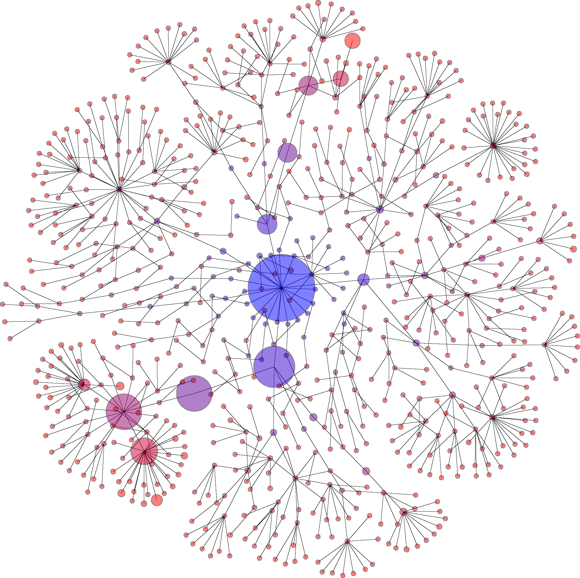
(We can adjust the gravity force by using the "Gravity adjust" slide bar under the "plot" menu in the demonstration).
To switch back to the constrained view, hit "T" on the keyboard (or click on the "arrange (entire tree)" button in the left control panel).
Another nice thing about the view is that we can drag individual sections of the tree to different regions of the screen. In the below view, we have dragged the node representing Proteobacteria to the corner of the screen. We then hit the "A" button (or click on the "arrange (around last selected)" button in the left control panel):
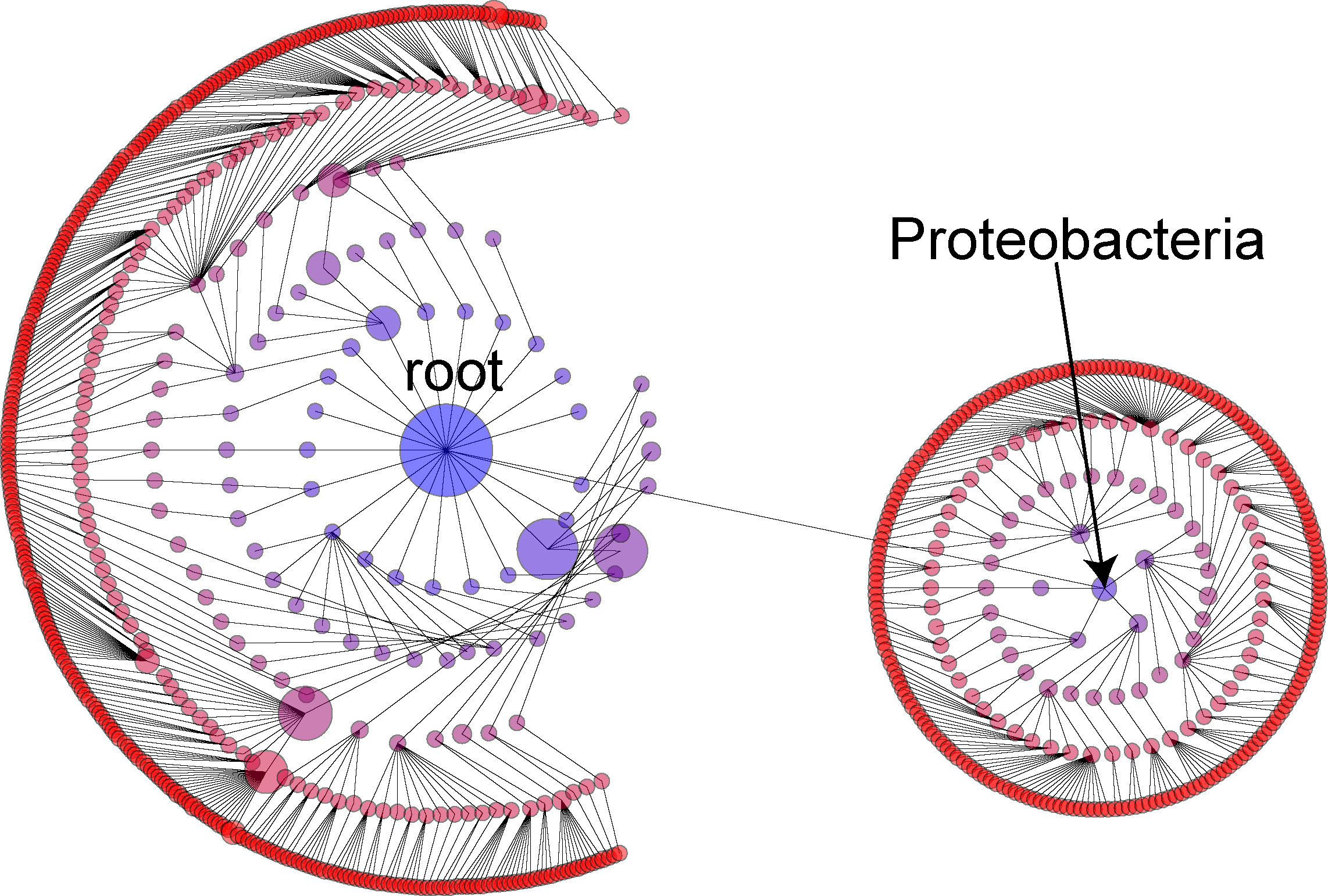
This allows us to break out sub-taxa that we are interesed in for a more detailed inspection than is possible
when the taxa is constrained by all of the other taxa in the tree.
(Hitting the "V" button repeatedly allows us to toggle between only showing the last selected).
We can use the interface to continue to break down our phylogenetic tree to any desired level of phylogenetic resolution. For example here we have created a third level for Gammaproteobacteria (by dragging the "Gammaproteobacteria" node to where we want it and again hitting "A")
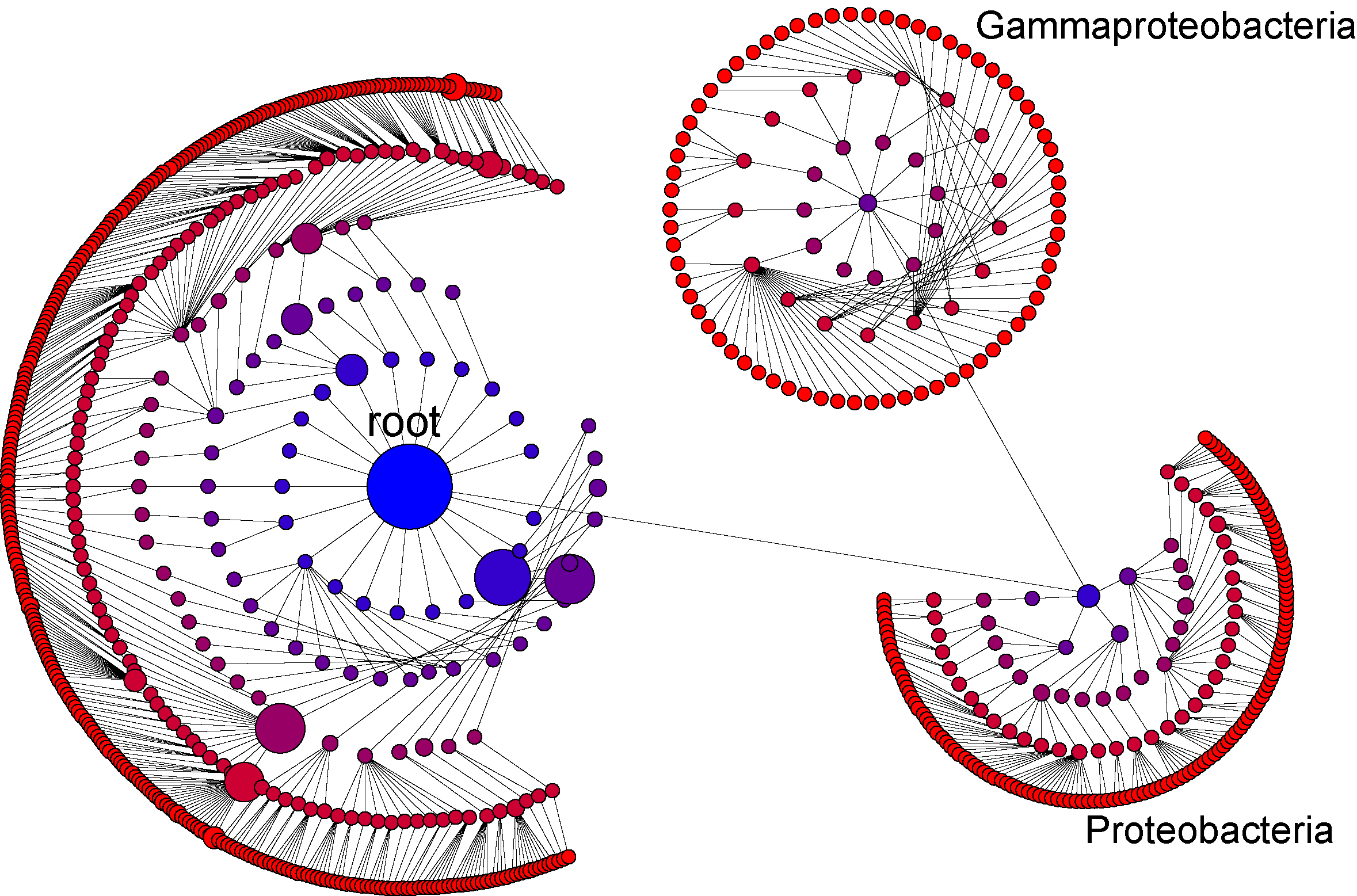
Having arranged the view in this way, we can switch to an inference driven view. By selecting "-log10TTestP" under size on the left control panel, we change the view so that the size of each node no longer reflect the number of sequences in each node, but rather the -log10(pValue) where pValue is the result of a t-test evaluating the null hypothesis that the distribution of each node is the same in case and control..

This allows us to visualize inference information in a way that is hierarchcially sensitive to
taxonomic information. Larger nodes are taxa that are more significantly different between case and control.
This is a rich visualization that will reveal patterns that may not be obvious when
considering taxomomic and inferential relationships separately. For example, order
Pasteurellales (inidcated by the arrow above) is more significantly different between case
and control than any mord derived taxa under Pasteurellales. By contrast, genus Sphingobium
(also indicated by an arrow ) is more significant than any of its parent taxa higher in the tree.
(We can view each branch of the tree separate from all other branches by toggling the v key)